Individual Ranking Criteria:

In these regards, ranking criteria, e.g., the one proposed in akhter2018empirical for various RDF partitioning techniques, helps provide a high-level view of the performance of a particular dimension across queries. Thus, we have extended the proposed ranking techniques to schemas and storage. The following equation shows a generalized formula for calculating ranking scores.

In the above equation, $R$ defines the Rank Score of the ranked dimension (i.e., relational schema, partitioning technique, or storage backend). Such that, d represents the total number of variants in the ranked dimension, O_dim(r) denotes the occurrences of the dimension being placed at the rank r (1st,2nd,..), While Q in the formula, represents the total number of query executions, as we have 11 query executions in our SP2Bench benchmark (i.e. Q=11).

Example of Calulating Rank Scores for the different dimensions:

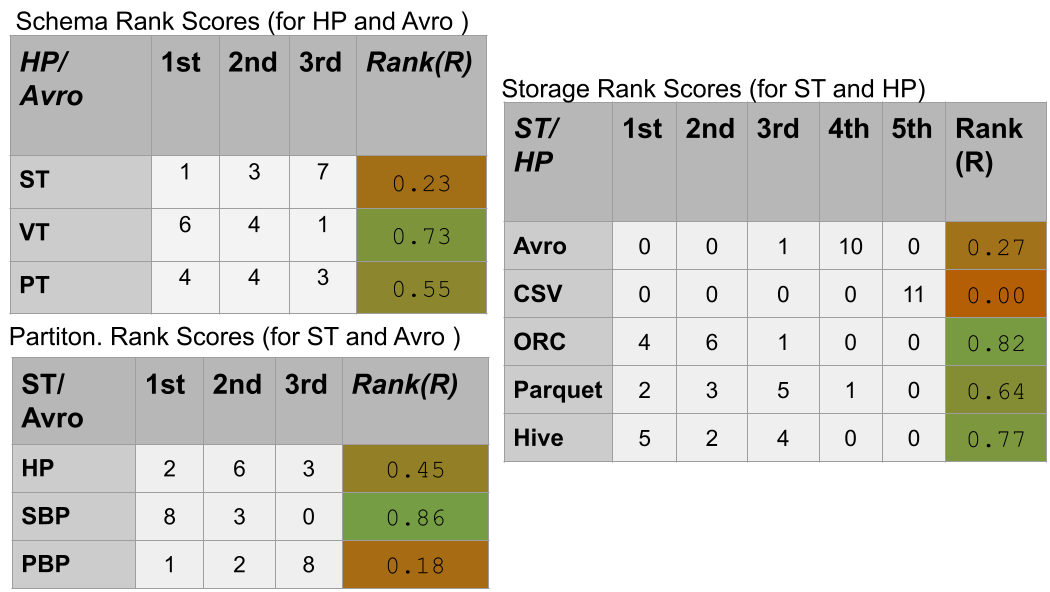
In the above example, each Rank Score (R) value for a dimension is calculated using the Equation (1). Let’s take an example, of calcuating R value for the ST relational schema. Out of the 11 Queries of the SP2Bench, the ST schema acheived the 1st place (i.e according to Avg. execution runtimes) 1 time, the 2nd rank 3 times, and as the 3rd ranked relational schema 7 times. Thus, the calcuation of the equation for ST (Partitioned Horizontally, and Stored as in HDFS Avro backend).

$R_s(ST)=\sum_{r=1}^{3}\frac{O_{dim}(r)*(3-r)}{11*(3-1)} =\frac{1*(3-1)+3*(3-2)+7*(3-3)}{22}=~0.23$

Similarly, VT, and PT schemata are ranked using the above equation, but according to their 1st, 2nd, and 3rd occurences, they have differnt Rank-Score values of 0.73, 0.55, respectively.

Note: When we apply the generalized ranking formula in Equation (1), we get three rankings for our three mentioned experimental dimensions (Relational Schemata; Partitioning, and Storage Backends), namely, “R_s” , “R_p”, and “R_f” accordingly.

Applying the above ranking function for the three dimensions, we get rank scores for the three diemsnions. In particular, we pivot on a “single dimension” options/alternatives and get scores for those alternatives (Schema options are »ST, VT, and PT), across the other two dimensions (partioning and storage if we rank schema).
Figures of ranking can be found here, specifically under the (Single-dimensional “Bench-Ranking”).
Please notice that Previously, we run experiments that include “Hive” as a 5^th storage backend, Therefore, we put both pile of figures that include Hive and the ones that exclude it for the three datasets (100M, 250M, and 500M).

Single-dimensional Ranking Criteria (R_s, R_p, and R_f) challenges:

Applying the ranking criteria independently for each dimension supports explanations of the results [5]. Nevertheless,we observed that ranking prescriptions are incoherent across dimensions. The most reasonable explanation is that these mono-dimensional ranking criteria can not capturea general view, leading to decisive trade-offs.

Example that shows the trade-offs among our problem experimental dimensions:

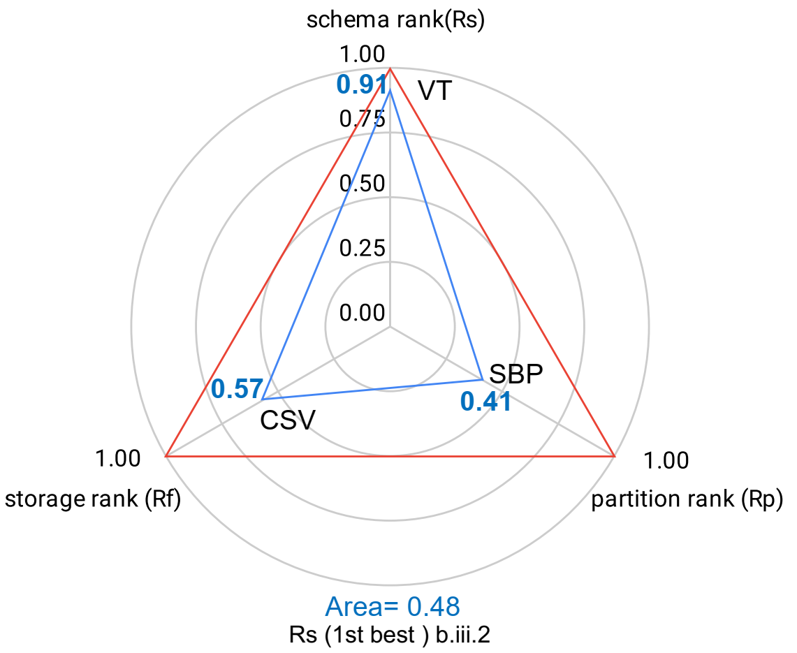
The following table shows the best three-ranked configuration combinations. The ”best-ranked” means the configuration combination that shows the highest rank score according to each ranking criterion (R_s, R_p, and R_f). Looking at the table, we observe that ranking over one of the dimensions provides a better insight for the decision maker.

Top-3 Configurations	100M			250M			500M
Rs	b.iii.2	b.iii.1	b.iii.4	b.iii.1	b.iii.2	b.iii.3	b.iii.1	b.iii.2	b.iii.4
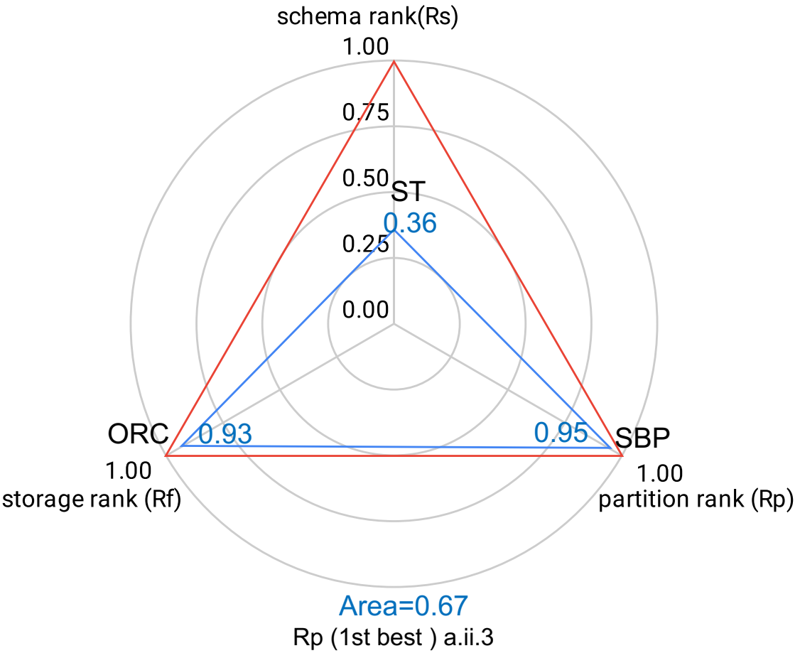
Rp	a.ii.3	a.ii.4	a.ii.5	a.ii.5	b.ii.3	c.ii.3	c.ii.3	c.ii.4	b.ii.5
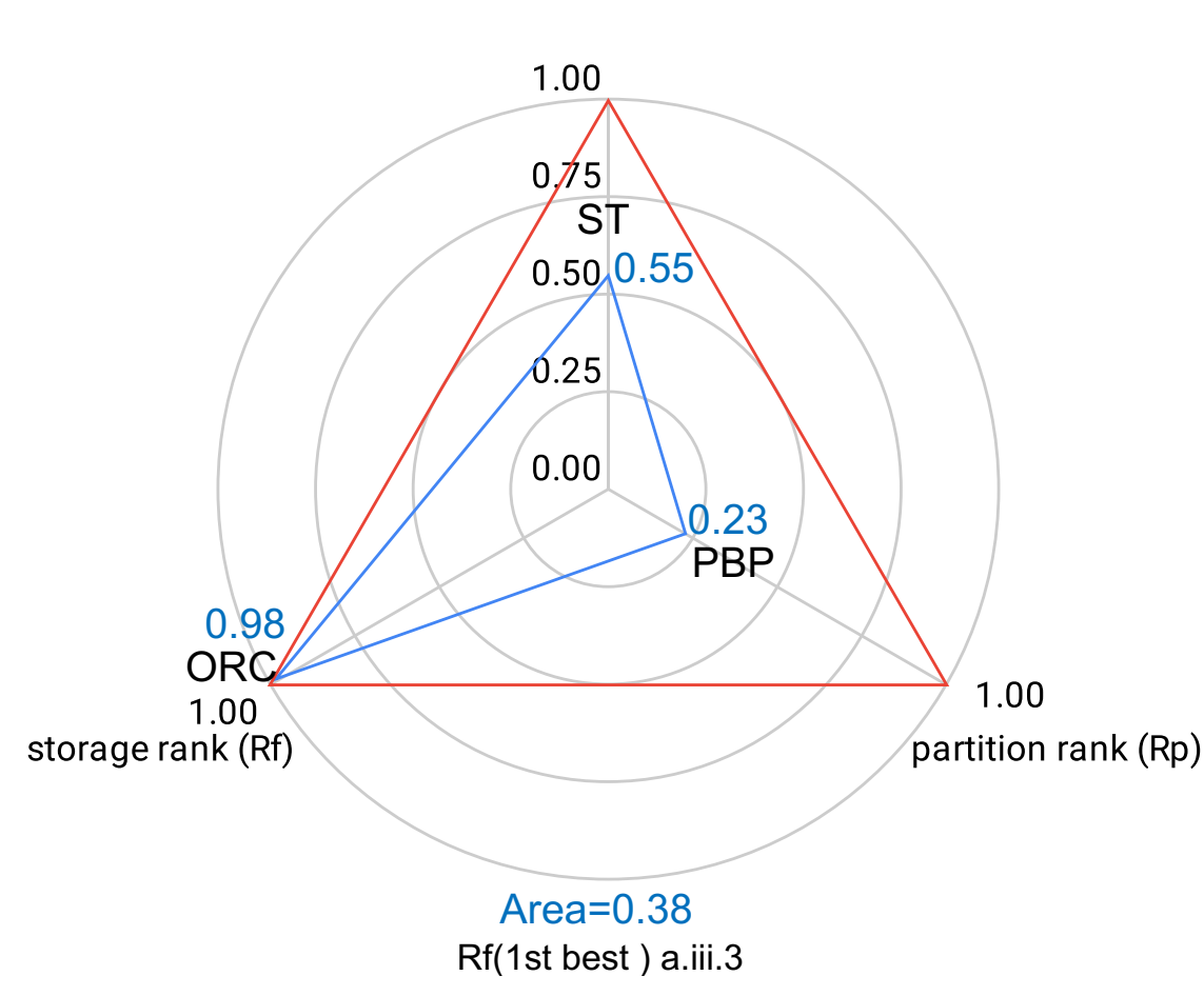
Rf	a.iii.3	a.ii.3	c.ii.3	a.iii.3	a.ii.3	b.ii.4	a.ii.3	a.iii.3	b.i.4

Indeed, for each dimension and across scalable datasets, we can mark the best performing dimension.

For example, ranking by the dimension of schema, we can mark VT (b) as the best.
While ranking by partitioning, we can mark the SBP (ii) as the best performing.
Last but not least, we can mark roughly that ORC(3) followed by Parquet(4) are the best storage backends.

Nevertheless, ranking over one dimension and ignoring the others ends up with selecting different configurations. For instance, ranking over R_s, i.e.,relational schema; R_p, i.e., partitioning technique, or R_f, i.e., the storage backend, end up selecting different combinations of schema, partitioning and storage backends.

In the following figure, we show the separate ranking criteria wrt the geometrical representation of the ranking criteria dimensions. The “Blue triangles” in the plots represent the actual optimization achieved by each ranking criteria.

Figures show that separate ranking criteria only optimize one dimension, maximizing the corresponding rank, while other dimensions can have non-optimal rank scores.

SPARKSQL RDF Benchmark.