SPARKSQL RDF Benchmark.
A systematic Benchmarking on the performance of Spark-SQL for processing Vast RDF datasets
- Home
- Bench-Ranking
- Ranking Criteria
- Ranking Goodness
- Project Source Code
- Results
- Benchmark Datasets
- Download Logs
This project is maintained by DataSystemsGroupUT
Multi-Dimensional Ranking Criteria
The single-diemsnional ranking criteria give better explaininations than descriptive and diagnostic analysis. Indeed, they provide clear insights towards the ranked dimension. However, ranking over one dimension and ignoring the others ends up with selecting different configurations. This intuition leads to extend the Bench-ranking into a multiobjective optimization problem in order to optimize all the dimensions at the same time.
Bench-ranking as a MO optimization problem
In our experiments, we adopt the standard Pareto front optimization techniques to consider all the experimental dimension altogether. The Pareto front framework conducts the MO optimization over several dimensions in order to find the best possible parameter configurations for the learning outcome of the highest performance. In particular, we utilized the Non-dominated Sorting Genetic Algorithm (NSGA-II) as one of the most popular Pareto front algorithms in order to find the best configuration combinations in our complex experimental solution space. Furthermore, MO optimization techniques can handle any arbitrary number of dimensions and objective functions.
Multi-Dimensional Ranking Criteria in Paractice
In our experiments, we calculate the Pareto fronts for our Bench-Ranking problem in two ways.
The first way, which we call (ParetoQ), applied NSGA-II algorithm considering the rank sets obtained by sorting w.r.t each query result individually (see Table IV). The algorithm aims at minimizing the query runtimes globally.
The second way, called (ParetoAgg.), operates on the single-dimensional ranking criteria, i.e., Rs, Rp, and Rf . In this case, the algorithm aims at maximizing the performance of the three ranks altogether. Notably, for both implementations of the algorithm, the search space is given in the form of configurations’ query runtimes (configurations query positions, see Table IV), or in configurations’ rank scores (Rs, Rf , Rp) in the aggregated form of Pareto, instead of generating a search space.
Pareto Results
The following table shows the Pareto fronts for both approaches, i.e., non-dominated solutions, which correspond to the overall optimal configurations for the 100M, 250M, and 500M triples datasets.
| 100M | ||||||||||||||||||||
|---|---|---|---|---|---|---|---|---|---|---|---|---|---|---|---|---|---|---|---|---|
| Pareto_Agg | b.ii.4 | a.ii.3 | c.ii.3 | c.ii.4 | b.ii.1 | c.i.1 | c.i.4 | c.ii.2 | b.iii.1 | b.iii.2 | a.iii.3 | b.ii.2 | b.i.2 | - | - | - | - | - | - | - |
| Pareto_Q | b.ii.4 | b.ii.3 | b.i.4 | b.i.3 | b.ii.1 | c.ii.4 | a.ii.3 | c.ii.3 | b.i.1 | c.i.4 | c.i.3 | b.iii.4 | b.ii.2 | b.iii.3 | c.ii.2 | a.i.4 | c.i.2 | a.iii.3 | c.iii.3 | c.iii.4 |
| 250M | |||||||||||||||
|---|---|---|---|---|---|---|---|---|---|---|---|---|---|---|---|
| Pareto_Agg | b.ii.3 | b.ii.4 | b.iii.1 | c.ii.3 | a.ii.3 | a.iii.1 | - | - | - | - | - | - | - | - | - |
| Pareto_Q | b.ii.4 | b.ii.3 | b.iii.1 | b.iii.4 | b.iii.3 | c.ii.4 | c.ii.3 | c.i.4 | c.ii.1 | b.i.2 | c.ii.2 | c.i.2 | c.iii.1 | c.iii.4 | c.iii.3 |
| 500M | ||||||||||||||||
|---|---|---|---|---|---|---|---|---|---|---|---|---|---|---|---|---|
| Pareto_Agg | c.ii.4 | b.ii.4 | b.iii.1 | b.iii.3 | b.iii.4 | b.ii.3 | a.ii.3 | a.iii.3 | b.i.4 | - | - | - | - | - | - | - |
| Pareto_Q | b.ii.3 | b.ii.4 | b.iii.3 | b.iii.4 | b.i.3 | b.iii.1 | b.i.4 | b.ii.1 | c.ii.4 | c.ii.3 | a.ii.3 | c.i.3 | a.iii.3 | c.i.2 | c.ii.2 | c.iii.4 |
** Note that ‘-‘ means that those are the only solutions, no more.
- Our experiments results inrestingly show that ParetoQ gives always non-dominated solutions more than the aggregated version (ParetoAgg). Also, results show (tables above) that ParetoQ and ParetoAgg. solutions conform to each other, i.e., configurations suggested by ParetoAgg. are almost included in ParetoQ. Indeed, only 2 solutions out of 13 in ParetoAgg are not shown up in QueryRankings of ParetoQ in the 100M, 2 out of 6 , 0 out of 9 in the 250M , and 500M datasets, respectively.
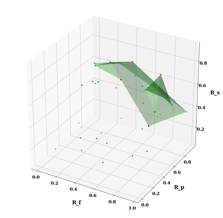
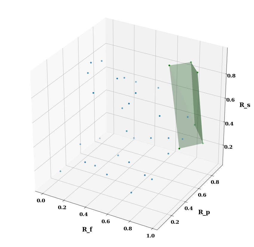
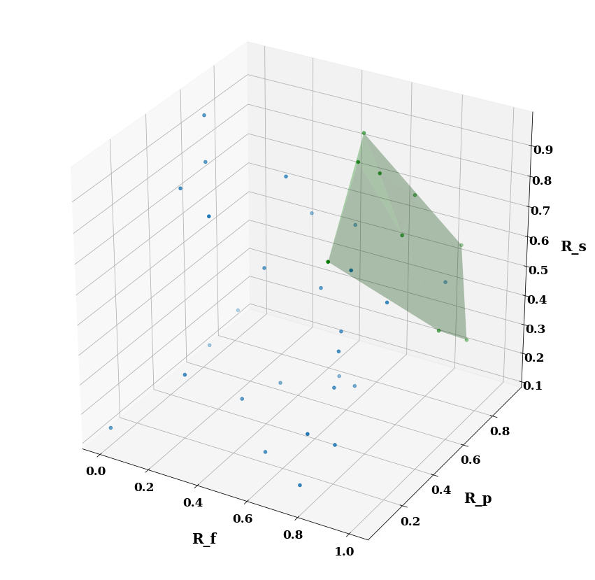
Pareto plots
The below figures (a), (b), and (c) show the Pareto fronts (depicted by the green shaded areas) of the three dimensions of the Bench-ranking for ParetoAgg. Each point of those figures represents a solution of rank scores (i.e, configuration in our case).